Improving RBMs with physical chemistry

Restricted Boltzmann Machines (RBMs) are like the H atom of Deep Learning.

They are basically a solved problem, and while of academic interest, not really used in complex modeling problems.  They were, upto 10 years ago, used for pretraining deep supervised nets.  Today, we can train very deep, supervised nets directly.

RBMs are the foundation of unsupervised deep learning–

an unsolved problem.

 RBMs appear to outperform Variational Auto Encoders (VAEs) on simple data sets like the Omniglot set–a data set developed for one shot learning, and used in deep learning research.

Omniglot Dataset

RBM research continues in areas like semi-supervised learning with deep hybrid architectures, Temperature dependence,  infinitely deep RBMs, etc.

Many of basic concepts of Deep Learning are found in RBMs.

Sometimes clients ask, “how is Physical Chemistry related to Deep Learning ?”

In this post, I am going to discuss a recent advanced in RBM theory based on ideas from theoretical condensed matter physics and physical chemistry,

the Extended Mean Field Restricted Boltzmann Machine: EMF_RBM

(see: Training Restricted Boltzmann Machines via the Thouless-Anderson-Palmer Free Energy ) 

[Along the way, we will encounter several Nobel Laureates, including the physicists David J Thouless (2016) and Philip W. Anderson (1977), and the physical chemist Lars Onsager (1968).]

RBMs are pretty simple, and easily implemented from scratch.  The original EMF_RBM is in Julia; I have ported EMF_RBM to python, in the style of the scikit-learn BernoulliRBM package.

Show me the code

https://github.com/charlesmartin14/emf-rbm/blob/master/EMF_RBM_Test.ipynb

Theory

We examined RBMs in the last post on Cheap Learning: Partition Functions and RBMs. I will build upon that here, within the context of statistical mechanics.

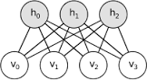
RBMs are defined by the Energy function

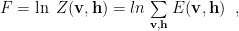
To train an RBM, we minimize the log likelihood ,

the sum of the clamped and (actual) Free Energies, where

and

The sums range over a space of  ,

which is intractable in most cases.

Training an RBM requires computing the log Free Energy; this is hard.

When training an RBM,  we

1. take a few ‘steps toward equilibration’, to approximate F
2. take a gradient step, , to get W, a, b
3. regularize W (i.e. by weight decay)
4. update W, a, b 
5. repeat until some stopping criteria is met

We don’t include label information, although a trained RBM can provide features for a down-stream classifier.

Extended Mean Field Theory:

The Extended Mean Field (EMF)  RBM is a straightforward application of known statistical mechanics theories.

There are, literally, thousands of papers on spin glasses.

The EMF RBM is a great example of how to operationalize spin glass theory.

Mean Field Theory

The Restricted Boltzmann Machine has a very simple Energy function, which makes it very easy to factorize the partition function Z , explained by Hugo Larochelle, to obtain the conditional probabilities

The conditional probabilities let us apply Gibbs Sampling, which is simply

• hold fixed, sample 
• hold fixed, sample 
• repeat for 1 or more equlibiration steps

In statistical mechanics, this is called a mean field theory.  This means that the Free Energy (in ) can be written as a simple linear average over the hidden units

.

where is the mean field of the hidden units.

At high Temp., for a spin glass, a mean field model seems very sensible because the spins (i.e. activations) become uncorrelated.

This is non-trivial to prove

Theoreticians use mean field models like the p-spin spherical spin glass to study deep learning because of their simplicity.  Computationally, we frequently need more.

How we can go beyond mean field theory ?

The Onsager Correction

Onsager was awarded 1968 the Nobel Prize in Chemistry for the development of the Onsager Reciprocal Relations, sometimes called the ‘4th law of Thermodynamics’

The Onsager relations provides the theory to treat thermodynamic systems that are in a quasi-stationary, local equilibrium.

Onsager was the first to show how to relate the correlations in the fluctuations to the linear response.  And by tying a sequence of quasi-stationary systems together, we can describe an irreversible process…

..like learning.  And this is exactly what we need to train an RBM.

In an RBM, the fluctuations are variations in the hidden and visible nodes.

In a BernoulliRBM, the activations can be 0 or 1, so the fluctuation vectors are

The simplest correction to the mean field Free Energy, at each step in training, are the correlations in these fluctuations:

where W is the Energy weight matrix.

Unlike normal RBMs, here is we work in an Interaction Ensemble, so the hidden and visible units become hidden and visible magnetizations:  

To simplify (or confuse?) the presentations here, I don’t write magnetizations (until the Appendix).

The corrections make sense under the stationarity constraints, that the Extended Mean Field RBM Free Energy () is at a critical point

,

That is, small changes in the activations do not change the Free Energy.

We will show that we can write

as a Taylor series in , the inverse Temperature, where  is the Entropy

,

is the standard, mean field RBM Free energy

,

and is the Onsager correction

.

Given the expressions for the Free Energy, we must now evaluate it.

Thouless-Anderson-Palmer TAP Theory

The Taylor series above is a result of the TAP theory — the Thouless-Anderson-Palmer approach developed for spin glasses.

 The TAP theory is outlined in the Appendix; here it is noted that

Thouless just shared the 2016 Nobel Prize in Physics (for his work in topological phase transitions)

Temperature Dependence and Weight Decay

Being a series in inverse Temperature , the theory applies at low , or high Temperature.   For fixed , this also corresponds to small weights W. 

Specifically, the expansion applies at Temperatures above the glass transition–a concept which I describe in a recent video blog.

Here, to implement the EMF_RBM, we set

,

and, instead, apply weight decay to keep the weights W from exploding

where may be an L1 or L2 norm.

Weight Decay acts to keep the Temperature high.

RBMs with explicit Temperature

Early RBM computational models were formulated using statistical mechanics  (see the Appendix) language, and so included a Temperature parameter, and were solved using techniques like simulated annealing and the (mean field) TAP equations (described below).

Adding  Temperature allowed the system to ‘jump’ out of the spurious local minima.  So any usable model required a non-zero Temp, and/or some scheme to avoid local minima that generalized poorly.  (See:  Learning Deep Architectures for AI, by Bengio)

These older approaches did not work well –then — so Hinton proposed the Contrastive Divergence (CD) algorithm.  Note that researchers struggled for some years to ‘explain’ what optimization problem CD actually solves.

More that recent work on Temperature Bases RBMs also suggests that higher T solutions perform better, and that

 “temperature is an essential parameter controlling the selectivity of the firing neurons in the hidden layer.”

Training without Sampling:  Fixed Point equations

Standard RBM training approximates the (unconstrained) Free Energy, F=ln Z, in the mean field approximation, using (one or more steps of) Gibbs Sampling.  This is usually implemented as Contrastive Divergence (CD), or Persistent Contrastive Divergence (PCD).

Using techniques of statistical mechanics, however, it is possible to train an RBM directly, without sampling, by solving a set of deterministic fixed point equations.

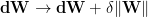
Indeed, this approach clarifies how to view an RBM as solving a (determinisitic) fixed point equation of the form

Consider each step, at at fixed (), as a Quasi-Stationary system, which is close to equilibrium, but we don’t need to evaluate ln Z(v,h) exactly.

We can use the stationary conditions to derive a pair of coupled, non-linear equations

They extend the standard formula of sigmoid linear activations with additional, non-linear, inter-layer interactions.

They differs significantly from (simple) Deep Learning activation functions because the activation for each layer explicitly includes information from other layers.

This extension couples the mean () and total fluctuations () between layers.  Higher order correlations could also be included, even to infinite order, using techniques from field theory.

We can not satisfy both equations simultaneously, but we can satisfy each condition individually, letting us write a set of recursion relations

These fixed point equations converge to the stationary solution, leading to a local equilibrium.  Like Gibbs Sampling, however,  we only need a few iterations (say t=3 to 5). Unlike Sampling, however, the EMF RBM is deterministic.

Implementation

• The original implementation of the EMF-RBM is in the Sphinx Team Julia package Boltzmann.jl
• I have ported the second order EMF-RBM to python, in the style of the scikit learn BernoulliRBM package.  The python code is available at

https://github.com/charlesmartin14/emf-rbm/

If there is enough interest, I can do a pull request on sklearn to include it.

The next blog post will demonstrate how the python code in action.

Appendix

the Statistical Mechanics of Inference

Early work on Hopfield Associative Memories

Most older physicists will remember the Hopfield model.  They peaked in 1986, although interesting work continued into the late 90s (when I was a post doc).

Originally, Boltzmann machines were introduced as a way to avoid spurious local minima while including ‘hidden’ features into Hopfield Associative Memories (HAM).

Hopfield himself was a theoretical chemist, and his simple model HAMs were of  great interest to theoretical chemists and physicists.

Hinton explains Hopfield nets in his on-line lectures on Deep Learning.

The Hopfield Model is a kind of spin glass, which acts like a ‘memory’ that can recognize ‘stored patterns’.  It was originally developed as a quasi-stationary solution of more complex, dynamical models of neuronal firing patterns (see the Cowan-Wilson model).

Early theoretical work on HAMs studied analytic approximations to ln Z to compute their capacity (), and their phase diagram.  The capacity is simply the number of patterns   a network of size N can memorize without getting confused.

Phase diagram of a Hopfield Network

The Hopfield model was traditionally run at T=0.

Looking at the T=0 line, at extremely low capacity, the system has stable mixed states that correspond to ‘frozen’ memories.  But this is very low capacity, and generally unusable.  Also, when the capacity too large, , (which is really not that large),  the system abruptly breaks down completely.

There is a small window of capacity, ,with stable pattern equilibria, dominated by frozen out, spin glass states.   The problem is, for any realistic system, with correlated data, the system is dominated by spurious local minima which look like low energy spin glass states.

So the Hopfield model suggested that

glass states can be useful minima, but

we want to avoid low energy  (spurious) glassy states.

One can try to derive direct mapping between Hopfield Nets and RBMs (under reasonable assumptions). Then the RBM capacity is proportional to the number of  Hidden nodes.    After that, the analogies stop.

The intuition about RBMs is different since (effectively) they operate at a non-zero Temperature.  Additionally, it is unclear to this blogger if the proper description of deep learning is a mean field spin glass, with many useful local minima, or a strongly correlated system, which may behave very differently, and more like a funneled energy landscape.

Thouless-Anderson-Palmer Theory of Spin Glasses

The TAP theory is one of the classic analytic tools used to study spin glasses and even the Hopfield Model.

We will derive the EMF RBM method following the Thouless-Anderson-Palmer (TAP) approach to spin glasses.

On a side note he TAP method introduces us to 2 more Nobel Laureates:

• David J Thouless, 2016 Nobel Prize in Physics
• Phillip W Anderson, 1977 Nobel Prize in Physics

The TAP theory, published in 1977, presented a formal approach to study the thermodynamics of mean field spin glasses.  In particular, the TAP theory provides an expression for the average spin

where is like an activation function, C is a constant, and the MeanField and Onsager terms are like our terms above.

In 1977, they argued that the TAP approach would hold for all Temperatures (and external fields), although it was only proven until 25 years later by Talagrand.  It is these relatively new, rigorous approaches that are cited by Deep Learning researchers like LeCun , Chaudhari, etc.    But many of the cited results have been suggested using the TAP approach.  In particular, the structure of the Energy Landscape, has been understood looking at the stationary points of the TAP free energy.

More importantly, the TAP approach can be operationalized, as a new RBM solver.

The TAP Equations

We start with the RBM Free Energy .

Introduce an ‘external field’ which couples to the spins, adding a linear term to the Free Energy

Physically,  would be an external magnetic field which drives the system out-of-equilibrium.

As is standard in statistical mechanics, we take the Legendre Transform,  in terms of a set of conjugate variables .  These are the magnetizations of each spin under the applied field,  and describe how the spins behave outside of equilibrium

The transform which effectively defines a new interaction ensemble .  We now set , and note

Define an interaction Free Energy to describe the interaction ensemble

which equals the original Free Energy when .

Note that because we have visible and hidden spins (or nodes), we will identify magnetizations for each

Now, recall we want to avoid the glassy phase; this means we keep the Temperature high.   Or  low.

We form a low Taylor series expansion  in the new ensemble

which, at low order in , we expect to be reasonably accurate even away from equilibrium, at least at high Temp.

This leads to an order-by-order expansion for the Free Energy .  The first order () correction is the mean field term.  The second order term () is the Onsager correction.

Second Order Free Energy

Upto , we have

or

Stationary Condition

Rather than assume equilibrium, we assume that, at each step during inference –at fixed (–the system satisfies a quasi-stationary condition.  Each step reaches a a local saddle point in phase space, s.t.

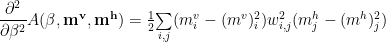
Stationary Magnetizations

Applying the stationary conditions lets us write coupled equations for the individual magnetizations that effectively define the (second order), high Temp, quasi-equilibrium states

Notice that the resemble the RBM conditional probabilities; in fact, at first order in , they are the same.

Mean Field Theory

 gives a mean field theory, and

And in the late 90’s, mean field TAP theory was attempted, unsuccessfully,  to create an RBM solver.

Fixed Point Equations

At second order, the magnetizations are coupled through the Onsager corrections.  To solve them, we can write down the fixed point equations, shown above.

Higher Order Corrections

We can include higher order correction the Free Energy by including more terms in the Taylor Series. This is called a Plefka expansion.  The terms can be represented using diagrams

Plefka (Diagrammatic) Expansion for the Free Energy

Plefka derived these terms in 1982, although it appears he only published up to the Onsager correction; a recent paper shows how to obtain all high order terms.

The Diagrammatic expansion appears not to have been fully worked out, and is only sketched above.

I can think of at least 3 ways to include these higher terms:

• Include all terms at a higher order in .   The Sphinx Boltzmann.jl packages includes all terms up to .  This changes both the Free Energy and the associated fixed point equations for the magnetizations.

Third Order Corrections

Fourth Order Corrections

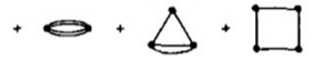
• Resum all diagrams of a certain kind. This is an old-school renormalization procedure, and it would include an  number of terms.   This requires working out the analytic expressions for some class of diagrams, such as all circle (RPA-like) diagrams

  

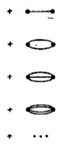
  all circle diagrams

  This is similar, in some sense, to the infinite RBM by Larochelle, which uses an resummation trick to include an infinite number of  Hidden nodes.

• Use a low order Pade Approximant, to improve the Taylor Series.   The idea is to include higher order terms implicitly by expanding the Free Energy as a ratio of polynomial functions  P, Q

 , where

,

Obviously there are lots of interesting things to try.

Beyond Binary Spins; Real-Valued RBMs

The current python EMF_RBM only treats binary data, just like the scikit learn BernoulliRBM.  So for say MNIST, we have to use the binarized MNIST.

There is some advantage to using Binarized Neural Networks on GPUs.

Still, a non-binary RBM may be useful.  Tremel et. al. have suggested how to use real-valued data in the EMF_RBM, although in the context of Compressed Sensing Using Generalized Boltzmann Machines.